10/15/2013

Creating A-nets

In this little post I will explain how to use VaryLab to create an A-net, i.e., a mesh with the property that each node and its neighbors lie in one plane.


Since A-nets are discrete versions of parametrization along asymptotic lines which only exist for surfaces with negative Gaussian curvature, we need to create a mesh with negative curvature first.

We start with a standard quad grid from the generators menu.
To obtain the right combinatorial structure, i.e., mesh topology,  we need to un-check the "Use Diamonds" box.

After clicking "Ok" we have a nice 6x6 quad grid.


Now we use the Vertex Coordinate Editor to move the corners of the grid up and down respectively. To do so we hold down the Shift key and the left mouse button and move the corners up and down.


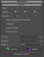
We fix the corners by selecting them with a left mouse click (the selected nodes are shown in red). Then we turn to the Optimizer Plugins panel and select Spring Energy. We select the const. option and set the target length to 0. This will make the edge behave like rubber bands/spring with 0 rest length. As optimization method I selected CG (Conjugate gradient) and maximal number of iterations 100. Finally we fix the selected points in the constraints panel by checking x, y, and z. Now we press the Optimize button to proceed with the optimization. And obtain a mesh with negative curvature.


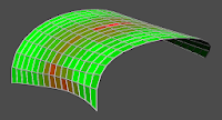
To turn this mesh into an A-net we use the Planar Vertex Stars optimizer from the Optimizer Plugin panel and optimize again. The mesh does not change a lot, since the above mesh is already almost an A-net after the first optimization.


8/28/2013

VaryLab Grasshopper Components

We started to implement a set of Grasshopper components to connect the VaryLab main program to the Rhino world. This is different to the prior approach of implementing a native Rhino 3D plug-in described in this article. Visit the download section to get the current version of the Grasshopper assembly.

The idea is to have a component that takes a mesh and uses a running VaryLab application to do the optimization. The resulting mesh is then delivered back to the component and written t the output of the component. Here is an example setup using the Optimization component.
A second component feeds the active geometry loaded in VaryLab into Grasshopper. This example brings the active VaryLab geometry into Grasshopper and scales it.
We plan to include more features. Planned are:

  • Storage of the VaryLab configuration as a Grasshopper component state
  • Configuration of boundary conditions through Grasshopper 
  • Expose more features like parametrization or remeshing

7/27/2013

VaryLab Cloud Models

The model manager
A new feature has arrived: VaryLab Cloud Models

Select the models section from the menu bar of the members area. This brings you to the models manager. Here you can upload and manage your own models and view shared models by other users.

Your own models can be shared with other users. Enter the email address of your partner in the add share section to create a new shared model with this person.

Your models can be used in VaryLab quite naturally. Just select a model from the corresponding project to load it at startup.

Model upload dialog
Per project model selection


7/01/2013

Discrete Surface Parameterization

When speaking about parameterization of a discrete surface we really mean the assignment of texture coordinates to the vertices of a mesh in VaryLab. This enables us to draw images on the surface and do processing in this image space. We can do re-meshing by introducing new vertices at some locations on the mesh guided by some pattern in texture space, e.g., a quad or triangle pattern. See this post for a description of the re-meshing capabilities of VaryLab. 

Default Settings


VaryLab supports a parameterization scheme called discrete conformal parameterization for triangle meshes. We implement an algorithm recently published here
To parameterize a mesh conformally in VaryLab you  press the "Unwrap" button in the Discrete Conformal Parameterization panel. There are a number of settings that define how the parameterization algorithm treats your mesh. The default settings should work well for triangle meshes that have one boundary component as in these pictures. These settings create a geometry in texture space where the edge lengths of the boundary edges are the same as in the mesh's geometry.

Textures In VaryLab


VaryLab supports the display of textures on meshes that are parameterized. You can select a texture from the "Content Appearance" panel. The default textures included in VaryLab are the re-meshing preview patterns quads, triangles, and hexagons. You can adjust the scale, position, orientation, and shear of the texture. These texture settings work also as preview for the re-meshing processor of VaryLab.


Manual Boundary Conditions 

For meshes with one boundary component we can define more complex boundary conditions. For instance we could select four boundary vertices as the corners of a rectangle in texture space. For this you have to select the four boundary vertices and edit their properties in the "Custom Vertices" panel. Check the "Custom Theta" check box and set their value to 90 degree. The global boundary options in the Boundary panel should be set to Conformal and Straight. Hit the Unwrap button to create the parameterization.

6/22/2013

VaryLab Data Visualization

Data visualization is one of most important tasks when doing surface optimization. On the basis of the analysis of data on the surface we decide what parameters go into the optimization and how the optimization core is performing. In this post we introduce the basic visualization features of VaryLab to you.

Visualization Panel
In VaryLab data visualization comes as a build in tool-kit, the halfedge data visualization panel. The basic idea is that data sources provide data for the nodes of a surface. So there are data providers for vertices, or edges, or faces, or all at once. These data providers deliver their data to visualizers that in turn have sockets that take data for vertices, edges, or faces and create their visualization. Select a data source from the middle of the panel. In the right box the compatible visualizers are presented long with buttons for the suitable node type. Click the node type button to activate the corresponding visualizer for this type of nodes.
E.g., to show a face area visualization select the FaceArea data source and the blue face button next to the node colors visualizer. The active node colors visualizer is listed in the top-left box along with its options.

There are a number of basic data visualizers contained in the module set of VaryLab web service.

Node Colors

Face planarity visualization by node colors
Colored nodes are a very effective way to represent scalar data on nodes. The nodes are colored using a color map. We mostly use the hue and red green color maps. This visualizer should be used in conjunction with the histogram to connect the colors with the function values.

Colored Beads

Face planarity visualized by colored beads
Similar to the node colors this visualizer represents scalar functions on surface nodes. In addition to the color the size of the spheres indicate the value of the function. There are options to adjust the overall scale and the span of the sphere radii. As for the node colors the color map can be chosen.

Histogram

A face planarity histogram
The histogram shows a discrete density plot of scalar data on surface nodes. It is integrated in the visualization panel in a tab behind the configuration. The color map can be adjusted to match the colors of a colored nodes or colored beads visualizer. The number of bins that are used to create the density plot can be selected from the visualizer options.

Vector Data

Vector field visualization
Vector data on surface nodes can be displayed with this visualizer. In VaryLab this is mainly used for the visualization of principle curvature directions and their singularities.


6/20/2013

Remeshing with VaryLab

Input Surface
The term remeshing referes to the change of mesh connectivity while retaining the overall shape of the surface. This post should give you an impression of the remeshing features of VaryLab.

We start with a geometry that is based on a square and exhibits a "smooth" triangulated surface. This geometry is the result of a form-finding process calculating node positions for certain load-bearing conditions. This geometry acts shell-like under some assumptions and we want to change its mesh to a quad based mesh and to a regular triangulation.

Quads Preview Texture


You can download this model from here if you follow this tutorial step by step. The model comes readily equipped with texture coordinates so we can apply a texture image to it. How to calculate texture coordinates is another story that can also be achieved with VaryLab. This is the topic of another post.


VaryLab comes with its standard remeshing preview textures. They can be selected from the content appearance panel and are applied to all models. We use triangles, quads, and hexagons as remesh patterns. You can adjust size and rotation of the preview texture. In this example we want the new triangles, or quads to align with the boundary of the surface so we do not rotate.


Remeshing Panel
The next step is the actual remeshing process. In the remeshig panel select the pattern you want to apply and hit the remesh button. For this example we choose either triangles quantized or quads quantized. This means that no chopped elements will end up at the boundary.
Quantized Triangles Mesh
The result of the remeshing operation is a flat mesh with the right connectivity. Press lift/flat to bring the vertices onto the target geometry. If you press this button again you are back to a flat mesh. In this flat mode one can do intermediate editing steps that we do not need for this simple example.

Quantized Quads Mesh
It is also possible to remesh with hexagons using the triangle pattern and an extra editing step. In some cases your model contains cuts and the remesh pattern has so called singularities. VaryLab has methods to cope with these situations and we will cover these advanced methods in a different post.


We hope this post helps understanding the features of VaryLab a bit better. See you for the next tutorial post.

6/17/2013

VaryLab Optimization Kick-Start


VaryLab is all about mesh optimization, we say discrete surface optimization. That means we modify a given mesh to have minimal energy in a certain sense. The energy in question is a combination of energies that is usually defined on the vertex positions of the input mesh. This post shows you how to optimize a mesh with VaryLab. It is a very simple example that illustrates the basic steps.

1. Import and Analysis


In this example we optimize a planarity measure of quadrilateral faces. We start with a quad-mesh and a maximum relative face non-planarity of 8.1%. You can download the model here if you like to follow this example.


The Halfedge Data Visualization panel contains a data source for for planarity. You can add a node color visualizer and a histogram to the list of active visualizations. Here we adjust the color map to red-green for the node colors and the histogram such that we can compare the model and the values in the data view. The histogram visualizer has a parameter for the number of bins to use, we set it to 40.

The model is a bent and twisted part of cylinder with almost planar quadrilaterals on the top and non-planar quad at the boundary. We have to decide on the goals of the optimization. In this case we want to keep the structure of the mesh and modify positions of all vertices.


2. Optimization Configuration


To begin optimization of the active mesh we have to select the energies that contribute to the energy used by the optimization core. The optimizer plug-ins panel holds a list of all available energies. If you use VaryLab online service you probably have only the energies you selected before startup. In this case we select the planar quads energy and choose the volume variant from the options. This energy is the sum of the volumes of tetrahedra spanned by non-planar quadrilaterals. This sum is scaled to render the energy scale invariant.

From the optimization panel we open the constraints sub-panel and uncheck all constraints especially the boundary should be variable. You can constrain the optimization to move the vertices only in the allowed coordinate directions. There are other more advanced constraints that can be enabled.
A tolerance of -8 lets the optimization core optimize the energy such that the gradient norm is less than \(10^{-8}\). The number iterations stops the optimizer after the given number of optimization steps. This number depends very much on the optimization method you select in the next box. There are methods that converge slowly but achieve nicer results than other methods that minimize the energy more rapidly. In the example we choose CG as the optimization method and a number of 180 iterations to perform.


 3. Optimization

To start the optimization hit the optimize button. A new optimization job is queued in the list of jobs and started if no other jobs are waiting to be executed. You can review and manage jobs in the job monitor. Here any pending and currently running optimization job can be cancelled. The progress bar of the optimization job shows the current iteration that is performed by the optimization core. It is possible to preview the shape of the model during optimization. The animate button starts a animated optimization job that updates the positions of vertices during optimization.

During optimization you can watch the optimization core doing its work in the optimization protocol panel. This panel shows a graph for every energy that is selected for optimization. Additionally, the norm of the gradient is plotted. From this information you can decide how the optimization is performing and if parameters should be adjusted. In our example we need approimately 100 iteration for the energy to drop below \(10^{-6}\) and 80 more iterations for the optimization to converge.

After optimization has finished the new model is shown in the view and data visualizers are updated to reflect new data. One can see for our model that optimization has changed the boundary shape drastically and faces are perfectly planar up to a tolerance of 0.02% for the most non-planar quad.

6/16/2013

VaryLab Usage 101

When using VaryLab for the first time the handling might seem a little unorthodox to people. I give a VaryLab usage 101 here to get you started frictionless.

1. Model Import/Export

We support a variety of file formats. To be precise we use the library jReality and its file reading and writing capabilities. The most robust format we use and recommend to you is OBJ. This can also be imported and exported by Rhinoceros 3D. It can be loaded and saved from the "Halfedge jReality Inteface" via the Import and Export buttons. This panel also supports layer management of meshes and layer mesh appearance properties.

2. Navigation


The most important commands are rotate, zoom, and fit. In the main tool bar you find buttons that en/disable the corresponding tools. Some specialities apply when using those tools. 
Rotate
The displayed model can be rotated by dragging on the background. The rotate tool is programmed to spin the model if you let the mouse button loose while dragging the cursor. This can be interrupted by clicking the scene background again without drag. 
Zoom
The zoom tool in the tool bar must be enabled in order to enable mouse wheel zoom. The fit or encompass tool does not respect the current zoom factor so you can always find the default view. 
Fit/Encompass
Encompassing or fitting the model is one of the most frequently used commands. Hit the 'e' key to fit the model to the view. If you zoomed your view this is not included. The encompass command can also be enabled in the main tool bar. 

3. Model Display

The display properties of your model are important, they define what features of your mode you see and how those are displayed. The appearance panel lets you edit many display parameters. A VaryLab model always consists of vertices, edges, and faces. The node visibility can also adjusted in the main tool bar.
Vertices
Hide or show the vertices of your model with the '1' key. Usually we display little spheres centered at the vertex locations. You can select vertices by click on these spheres. A second click deselected the vertex. Adjust the appearance or vertices in the global appearance panel. 
Edges
Hit the '2' key to show or hide edges of your model. Select edges with the mouse. 
Faces
The key for faces is the '3' key.

4. Editing

To edit a model you have to select some of its nodes. You can either click on a vertex, an edge, or a face to select, or you cn use the marquee tool to select a range of nodes from the model. Drag the mouse while holding down the Shift-Key selects vertices. With the ALT-KEY you select edges, and with the CTRL-Key faces are added to the selection. You can mix node types in the selection. To clear the selection, press CTRL-C. To delete nodes from the model just press DEL. There is a pop-up menu if right-click the view. Here you find further editing commands.

 I hope this will be some use to VaryLab beginners. Please ask questions if there are things unclear. 

6/15/2013

Rhino 4 and 5 Plug-Ins have arrived

The VaryLab plug-ins for Rhino3D 4 and 5 are ready. Rhino 4 32 Bit and Rhino 5 32/64 Bit are supported. We prepare a manual page for the user interface of the plug-in. You can download the plug-in files in the user area at http://my.varylab.com/#downloads.

6/13/2013

Spring Energy

The spring energy implemented in VaryLab comes with a few options that I want to explain here.
The user interface contains controls that adjust rest length to be constant length (const. option) , the original lenght (orig option), or rest range (range option) of springs. Every edge of the discrete surface is treated as a spring during optimization. In addition to setting a fixed length or range the optimizer can calculate the mean edge length of the mesh (avg. option) and use it as rest length of the springs. This mean can be automatically updated (update check box) when optimization starts. In a quad mesh the diagonals can be treated as springs (diagonals check box). The strength value is a coefficient of the energy when used in conjunction with other energies.

Stefan

6/12/2013

Module and Bundle Fixes

In the latest release we have included a few module structure updates and module bundle fixes. The planarization bundle now contains corresponding visualizer plug-ins. Optimization essentials are included in the planarization bundle. Default property files are used for newly created projects. And some more improvements and bug fixes. 

Stefan

5/25/2013

Approaching Feature Freeze

VaryLab Service is constantly evolving. We are now approaching a feature-freeze status. However for the beta phase there are some things yet to be implemented. Here is a list:

- example models for each bundle
- default property files for each bundle. 
- bundle blog pages need content. 
- issue tracker setup
- separate project configuration pages. 

The beta version release date is the
22th of Juli 2013
Save the date!

Stefan