3/31/2016

A new code signing certificate

As time goes by... Every couple of years we have to renew out code signing certificate for the java webstart version of VaryLab. This time has come again and it might come with problems for you when starting VaryLab. The caching of the webstart client seems to confuse things in some situations and may complain about signed jar files. To resolve this issue you will have to clear the application cache and remove VaryLab resources. Here is an example (in German) taken from MacOS:

Open the Java Cache Viewer
Delete the application
Delete any resources

2/16/2015

Optimization

In this post, we describe the different functionals available for discrete geometry optimization in VaryLab.

Circular Quads

Defines an energy functional which is minimal for planar circular quads. Since we are using an angle criterion, the convergence to planarity is relatively slow. If the planar quads energy is added to the optimization, the geometry converges more quickly.

Before


After


Incircle Quads

The property for a quadrilateral to possess an incircle tangent to its sides is that the two sums of opposite side lengths is equal $a+c=b+d$. Planarity is not included in this functional, so to get planar quadrilaterals with inscribed incircles you need to add planarity to the optimization.

Before


Optimized


Touching Incircles

In a quad-mesh with incircles, the incircles need not touch. So in combination with the incircles and planarity energies it one can create a mesh with touching incircles.
Before
Optimized


Conical

This energy implements an angle criterion for conical meshes. So in combination with planarity it optimizes a mesh to have the property, that faces adjacent to one node are tangent to a cone of revolution.


Direction Field

Allows the user to specify a direction field. This can be used with spring energy and boundary constraints to do simple form finding.


Equal Diagonals

The lengths of the diagonals of each quad are equal in an optimized mesh.


Planar Quads

A functional that forces planarity of quad faces


Planar Vertex Stars

This energy is dual to the planar faces energy. It computes the volume spanned by a node and its neighbors. Minimization yields meshes such that each node lies in a plane with its neighbors. If used together with face planarity the initial mesh is mapped to a plane.


Reference Mesh

Given a reference mesh we compute the closest point to a node and add a spring force between each node and its projection. The projection point is recomputed in each step of the optimization. If combined with other energies it keeps the optimized mesh close to a reference mesh.


Reference Surface

This is similar to Reference mesh but with a reference nurbs surface.


Spring Energy

The spring energy is computed by adding springs to all the edges of the mesh. These springs can have user specified target lengths and strengths that can be specified by various options.


Willmore Energy

See the article: A.I. Bobenko, A conformal energy for simplicial surfaces.


Parameterline Curvatures

There are many ways to define the curvature of a polygonal parameter line on a quad mesh. We have implemented a few different notions:


Geodesic Curvature

On smooth surface, the curvature of a surface curve is decomposed into geodesic and normal curvature, where geodesic curvature is the curvature in direction of the tangent plane. So we consider the projection of the parameter polyline into the tangent plane orthogonal to the normal at a node. For the optimized mesh, the projection is straight.


Opposite Angles Curvature

This curvature is based on the intrinsic geometry of the surface. Let $\alpha$, $\beta$, $\gamma$, and $\delta$ denote the angles in the adjacent quads at a node in cyclic order. Then the optimal mesh satisfies $\alpha+\beta = \gamma+\delta$ and $\beta+\gamma = \delta+\alpha$, i.e. so the parameter lines are straight from an intrinsic point of view.


Opposite Edges Curvature

This energy penalizes the deviation of a parameter polyline from a straight line. So using this energy only, will flatten the mesh to the plane. Used together with, e.g. a reference surface energy, this energy smoothes the  parameter lines of the quad mesh.


Circumcircle Curvature

The curvature is the inverse of the radius of the circle through three consecutive points on a parameter polyline.
Please leave a comment if you need you need more detailed information.
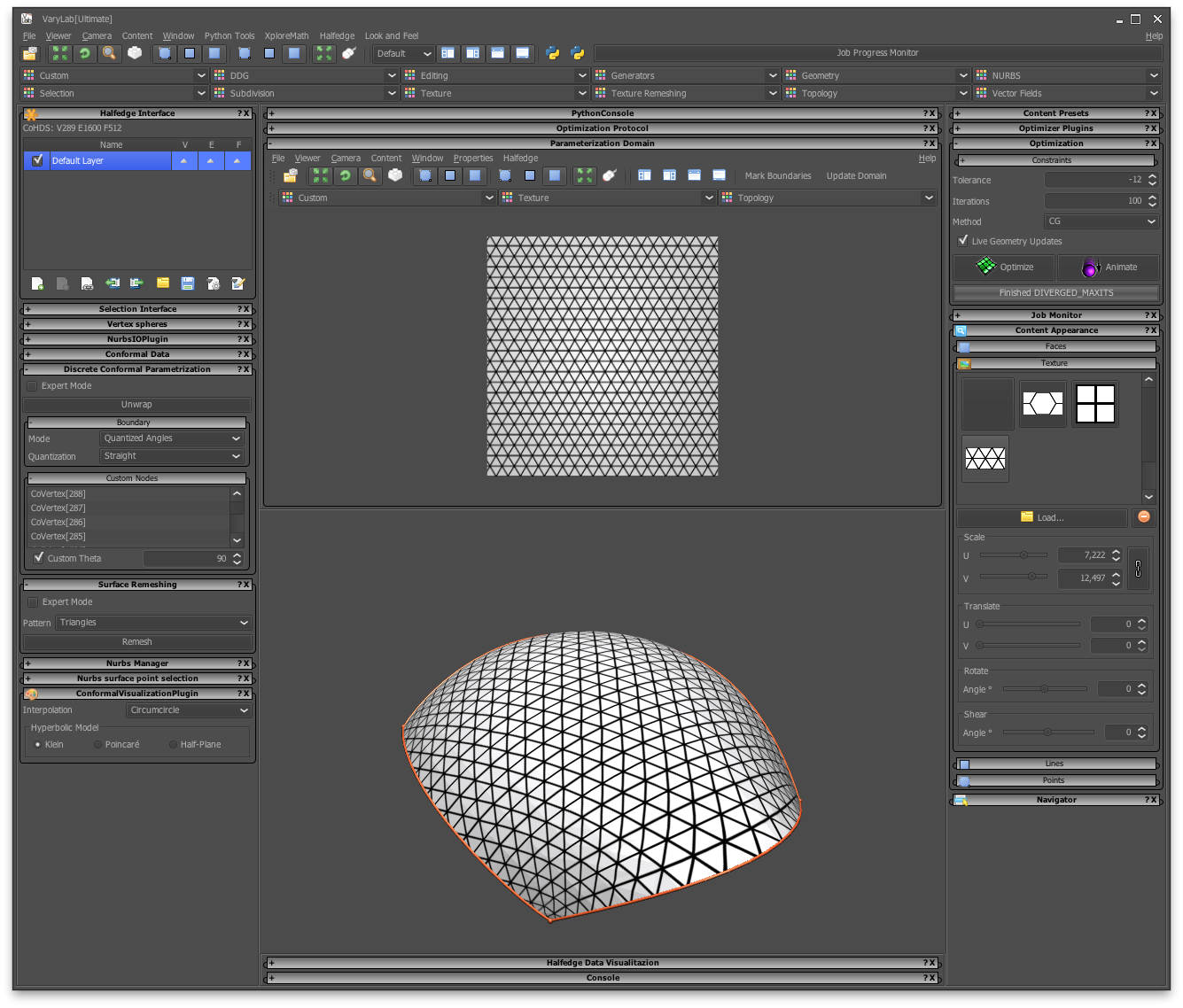
6/17/2014

Creating a Surface From Scratch

A minimal surface
In this post, we describe how VaryLab can be used to create a minimal surface from scratch. We use the build-in primitives of VaryLab to create a start geometry and modify this using interactive editing as well as tabular data input. Subdivision steps are used to obtain finer resolutions and to create the final mesh. This mesh is then optimized to have the shortest edge lengths possible with certain boundary conditions. This gives a coarse approximation of the shape of a minimal surface with the given boundary.

Creating a start geometry

The quad mesh generator dialog
We start by creating a simple square with a generator from the menu Generators->Quad Mesh. Set the u and v resolution to 2 and uncheck the "Use Dimonds" box. This creates our start geometry, a quadrilateral. You can move the vertices in space by selecting and Shift-Mouse-Drag
Initial quad-surface


An alternative way of coordinate input is the data table in the data visualization panel. You can activate the coordinate table by selecting the VPosition data channel and choose a table visualization for vertices. The table shows the coordinates of either all or just the selected vertices.

Linear subdivision surface
To obtain a finer surface resolution, we use several subdivision steps. From the menu choose Subdivision->CatmullClark. Here we can adjust subdivision parameters to create a linear subdivision and fixed boundary interpolation.

Coordinates can be edited in the data visualization panel

Adjust the position of vertices that should remain in a fixed location and keep them selected. The optimization can fix selected vertices in all or just some dimensions.


Optimization

Optimization user interface
The optimization core of VaryLab can be used to shorten the edge lengths of the mesh and keep certain vertices at fixed positions. The corresponding energy is the spring energy. Activate the Sping Energy optimizer from the Optimizer Plug-ins panel. The spring length should be set to constantly 0. In the Optimization panel you can select constraints. We fix all selected vertices. All other boundary vertices can move along the z-direction. To achieve this effect, check all boxes of the selection constraints and the x and the y check boxes of the boundary constraints.

To start the optimization you can either choose to interactively optimize by pressing the Animate button. Or you can optimize the mesh for a predefined number of steps with the Optimize button.

6/16/2014

Remeshing with Boundary Conditions

Initial Surface
A boundary of a discrete surface is usually a closed polygonal curve in space. If a surface has multiple boundary components, one speaks of a multiply-connected surface. In this article we deal with surfaces that have one boundary component. We call those simply-connected or surface with disk topology.

Source unstructured triangle mesh
Starting with a discrete surface with one boundary component we want to create a mesh where the pattern of the mesh aligns with the boundary curve in a nice way. You can download the example model here. We use a triangle pattern and demonstrate the usage of automatic as well as custom alignment of the boundary.

Boundary aligned parameterization

Custom boundary condtions
In order to create a new mesh from an existing surface, we first need to create a suitable parameterization for the input data. For general information about parameterization have a look into the Discrete Surface Parameterization article. In our case we want to create a parameterization that respects the geometry of a regular triangle pattern which means boundary angles of the domain of parameterization should be quantized to a multiple of 30º.

For the given triangulated surface, we create a map from the surface to a rectangle. In order to specify these boundary conditions, you select the four corner vertices of the mesh and type in the desired boundary angle in the "Custom Nodes" fold-out panel inside the "Discrete Conformal Parameterization" panel. If the vertices do not appear, press the Unwrap button and select the vertices again. To create the rectangle, the four vertices must have a custom angle of 90º. The general boundary setting should be set to "Quatized Angles" for the mode, and "Straight" for quantization. These settings affect all unselected vertices. If you press the unwrap button the mapping is calculated and can be previewed using the texture display features of VaryLab.

The VaryLab main window during parameterization. In 
the parameterization domain panel (top) you see can review the 
current domain. A texture is selected from the appearance panel
to preview the mapping.

Aligned Remeshing


Remeshing with boundary aligned
triangles
If we have a mesh with sufficiently quantized boundary angles, we can go on and create a boundary aligned mesh from this data. In our case we have four angles of 90º and at all other vertices the boundary of the domain is a straight line which corresponds to a boundary angle of 180º.

The remeshing user interface
To perform the remeshing step select the "Boundary aligned Triangles" pattern from the "Surface Remeshing" panel and hit the "Remesh" button. You can download the result mesh here.


10/15/2013

Creating A-nets

In this little post I will explain how to use VaryLab to create an A-net, i.e., a mesh with the property that each node and its neighbors lie in one plane.


Since A-nets are discrete versions of parametrization along asymptotic lines which only exist for surfaces with negative Gaussian curvature, we need to create a mesh with negative curvature first.

We start with a standard quad grid from the generators menu.
To obtain the right combinatorial structure, i.e., mesh topology,  we need to un-check the "Use Diamonds" box.

After clicking "Ok" we have a nice 6x6 quad grid.


Now we use the Vertex Coordinate Editor to move the corners of the grid up and down respectively. To do so we hold down the Shift key and the left mouse button and move the corners up and down.


We fix the corners by selecting them with a left mouse click (the selected nodes are shown in red). Then we turn to the Optimizer Plugins panel and select Spring Energy. We select the const. option and set the target length to 0. This will make the edge behave like rubber bands/spring with 0 rest length. As optimization method I selected CG (Conjugate gradient) and maximal number of iterations 100. Finally we fix the selected points in the constraints panel by checking x, y, and z. Now we press the Optimize button to proceed with the optimization. And obtain a mesh with negative curvature.


To turn this mesh into an A-net we use the Planar Vertex Stars optimizer from the Optimizer Plugin panel and optimize again. The mesh does not change a lot, since the above mesh is already almost an A-net after the first optimization.